Using the Quantum Audio Module
For building and manipulating quantum audio representations
The quantumaudio module implements a QuantumAudio class that is able to handle the encoding/decoding process of some quantum audio representations, such as: Building a quantum circuit for preparing and measuring the quantum audio state; simulating the circuit in Qiskit’s aer_simulator; running the circuit in real hardware using IBMQ (as long as you have an account, provider and backend); necessary pre and post processing according to each encoding scheme; plotting and listening the
retrieved sound.
The available encoding schemes are:
QPAM - Quantum Probability Amplitude Modulation (Simple quantum superposition or “Amplitude Encoding”) -
'qpam'SQPAM - Single-Qubit Probability Amplitude Modulation (similar to FRQI image representations) -
'sqpam'QSM - Quantum State Modulation (also known as FRQA) -
'qsm'
For more information regarding the representations above, you can refer to this book chapter, or its abridged pre-release draft in ArXiv
Using the package
First of all, make sure you have all of the following dependencies installed:
numpy
matplotlib
IPython.display
bitstring
qiskit
If you are on a Linux system, you might be able to install the dependencies by uncommenting and running this line:
[1]:
# !pip3 install numpy matplotlib ipython bitstring qiskit
If you have “pip installed” the quantumaudio module, it should have downloaded all of the required dependencies:
[2]:
# !pip3 install quantumaudio
[3]:
import numpy as np
import quantumaudio as qa
import matplotlib.pyplot as plt
from qiskit import QuantumCircuit, QuantumRegister, ClassicalRegister, Aer, execute
from qiskit.visualization import plot_histogram
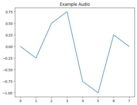
Then, we create/load some example digital audio. QPAM and SQPAM are representations that can handle arrays with floating point or decimal numbers from -1 to 1 (somewhat similar to a PCM .wav or .flac file). In this example, we are using an audio signal with 8 samples:
[4]:
digital_audio = np.array([0., -0.25, 0.5 , 0.75,  -0.75  ,  -1.,  0.25 ,  0.])
plt.plot(digital_audio)
plt.title("Example Audio")
plt.show()
This is the current workflow for using the quantumaudio module: The QuantumAudio class encapsulates everything, from input, preprocessing, circuit generation, qiskit jobs, audio reconstruction and output.
The user chooses which encoding technique to use while instantiating a QuantumAudio object. It will then refer to specific encoder subclass methods.
[5]:
# qsound = qa.QuantumAudio('ENCODONG_SCHEME_HERE')
After instantiation, the first method to be used load_input() will load a copy of the input audio inside the object. It will print out the space requirements of the circuit.
[6]:
qsound_qpam = qa.QuantumAudio('qpam')
qsound_qpam.load_input(digital_audio)

qsound_sqpam = qa.QuantumAudio('sqpam')
qsound_sqpam.load_input(digital_audio)
For this input, the QPAM representation will require:
         3 qubits for encoding time information and
         0 qubits for encoding ampĺitude information.
For this input, the SQPAM representation will require:
         3 qubits for encoding time information and
         1 qubits for encoding ampĺitude information.
[6]:
QuantumAudio
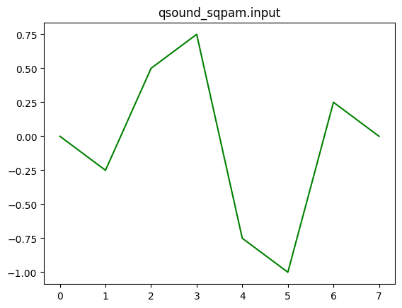
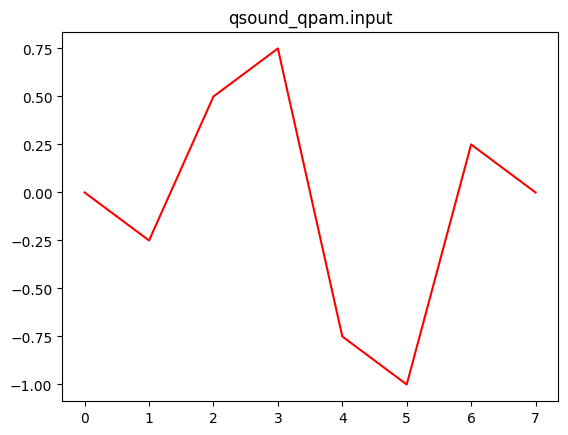
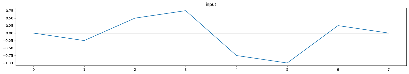
The loaded signal is acessible via the input attribute.
[7]:
plt.plot(qsound_qpam.input, 'r')
plt.title('qsound_qpam.input')
plt.show()
plt.plot(qsound_sqpam.input, 'g')
plt.title('qsound_sqpam.input')
plt.show()

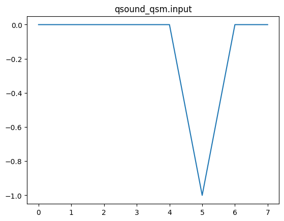
However, the same digital_audio example will NOT work with QSM. The QSM works with integer values only, as it expects a quantized signal, so it will round the numbers by default, removing all of the decimals and destroying the input, as shown:
[8]:
qsound_qsm = qa.QuantumAudio('qsm')
qsound_qsm.load_input(digital_audio)

plt.plot(qsound_qsm.input)
plt.title('qsound_qsm.input')
plt.show()
For this input, the QSM representation will require:
         3 qubits for encoding time information and
         1 qubits for encoding ampĺitude information.
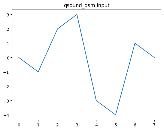
To load an input to the QSM encoder, we need to quantize (or re-quantize) the amplitudes of our signal. In this example, we have conveniently built a digital_audio simulating a PCM audio with 3-bit depth quantization. So we only need to multiply our signal by \(2^{bitDepth -1}\) and retrieve the quantized version of the signal:
[9]:
bit_depth=3
quantized_ditial_audio = digital_audio*(2**(bit_depth-1))

print(quantized_ditial_audio)
[ 0. -1. 2. 3. -3. -4. 1. 0.]
(To prove that this quantization also holds for actual sound files, uncomment the following block and load a typical 1 second of audio, 44100 Hz, 16-bit depth using and check. We used a CC sweep file found in Freesound.org (Note: For this tutorial, this file would be too large to simulate).
Also Note: this requires the soundfile package.
[10]:
# import soundfile as sf

# real_audio = sf.read('sweep_2_22000_log.wav')[0]

# bit_depth=16
# quantized_real_audio = real_audio*(2**(bit_depth-1))

# print(quantized_real_audio)
[ 0. 7. 13. ... -74. 38. 0.]
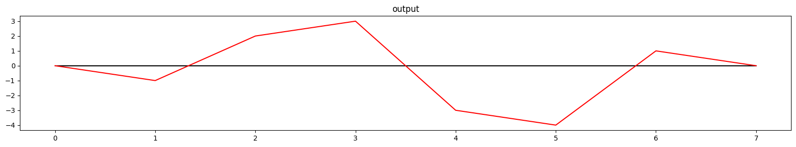
Now we can load the quantized version ou our example audio to QSM, by specifying the bit depth as an additional argument. Remeber that the bit deph will also dictate the amount of qubits necessary to store the amplitude information.
[11]:
qsound_qsm = qa.QuantumAudio('qsm')
qsound_qsm.load_input(quantized_ditial_audio, 3)

plt.plot(qsound_qsm.input)
plt.title('qsound_qsm.input')
plt.show()
For this input, the QSM representation will require:
         3 qubits for encoding time information and
         3 qubits for encoding ampĺitude information.
Note:
For usability reasons, QPAM and SQPAM can also handle quantized signals. The following code does exactly the same thing as before:
[12]:
# qsound__qpam = qa.QuantumAudio('qpam')
qsound_qpam.load_input(quantized_ditial_audio, 3)

# qsound_sqpam = qa.QuantumAudio('sqpam')
qsound_sqpam.load_input(quantized_ditial_audio, 3)

plt.plot(qsound_qpam.input, 'r')
plt.title('qsound_qpam.input')
plt.show()
plt.plot(qsound_sqpam.input, 'g')
plt.title('qsound_sqpam.input')
plt.show()
For this input, the QPAM representation will require:
         3 qubits for encoding time information and
         0 qubits for encoding ampĺitude information.
For this input, the SQPAM representation will require:
         3 qubits for encoding time information and
         1 qubits for encoding ampĺitude information.

This means that when working with quantized signals, we can easily switch between quantum audio representations - at least for encoding purposes (any additional quantum algorithm will have dramatically different impacts on each representation).
Now, let’s generate quantum circuits with 3 steps:
Converting/preprocessing the signal for a specified encoding scheme (for example, qpam converts the signal into probability amplitudes, sqpam creates an array of angles) - This is done internally by the QuantumAudio class when calling the
prepare()method.Generating a Preparation circuit for the input, which encodes the classical information into the quantum system acording to the representation - this is also done with the
prepare()method
(any custom quantum circuit, (aka, signal processing) could be applied at this point, by acessing the
circuitattribute - qsound.circuit)
Inserting measurement instructions at the end of the circuit - measure() method
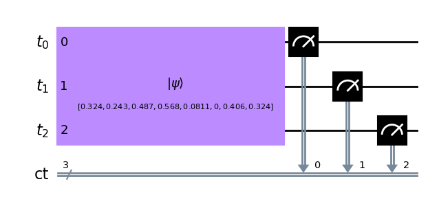
For now, we are only trying to prepare the quantum audio state and then measure it back: a Quantum Audio Bypass Circuit
[13]:
qsound_qpam.prepare()
qsound_qpam.measure()
qsound_qpam.circuit.draw('mpl')
[13]:
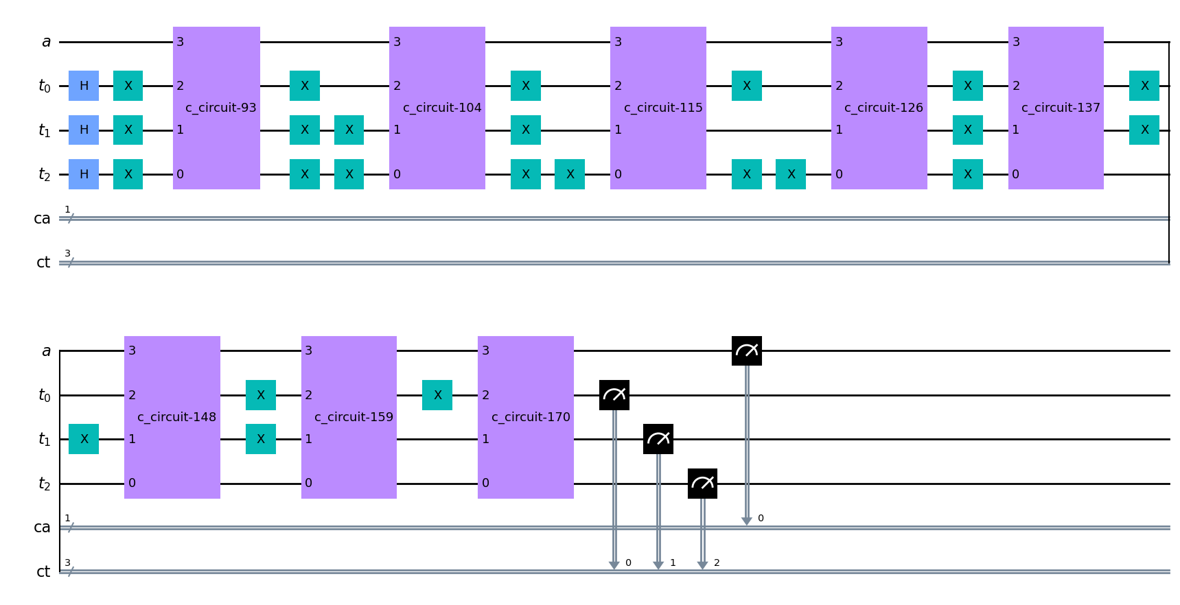
If you are a one-liner, fell free to write everything in a single line. This is the advantage of the QuantumAudio class, and may be very useful for live performances:
[14]:
qsound_sqpam.prepare().measure().circuit.draw('mpl')
[14]:
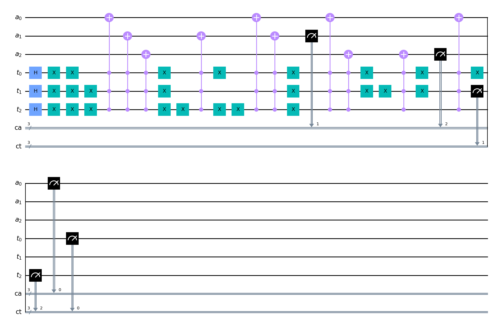
[15]:
qsound_qsm.prepare().measure().circuit.draw('mpl')
[15]:
Now that we have a quantum circuit, we can run it on aer_simutator, or use it elsewhere. There are attributes storing qiskit result and counts.
QPAM:
[16]:
# Default values: QuantumAudio.run(shots=10, backend_name='aer_simulator', provider=Aer)
# Simulating qsound_qpam.circuit in 'aer_simulator' with 1 thousand shots:
shots = 1000
qsound_qpam.run(shots)
print(qsound_qpam.result)
print('-----------------------------------')
print(qsound_qpam.counts)
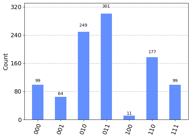
plot_histogram(qsound_qpam.counts)
Result(backend_name='aer_simulator', backend_version='0.11.1', qobj_id='e3d8679a-195a-42f5-9958-8a631e6459ec', job_id='48957fd5-50b4-49a1-bfbe-b90df251166c', success=True, results=[ExperimentResult(shots=1000, success=True, meas_level=2, data=ExperimentResultData(counts={'0x4': 11, '0x0': 99, '0x2': 249, '0x7': 99, '0x3': 301, '0x1': 64, '0x6': 177}), header=QobjExperimentHeader(clbit_labels=[['ct', 0], ['ct', 1], ['ct', 2]], creg_sizes=[['ct', 3]], global_phase=0.0, memory_slots=3, metadata={}, n_qubits=3, name='circuit-91', qreg_sizes=[['t', 3]], qubit_labels=[['t', 0], ['t', 1], ['t', 2]]), status=DONE, seed_simulator=2878838266, metadata={'noise': 'ideal', 'batched_shots_optimization': False, 'measure_sampling': True, 'parallel_shots': 1, 'remapped_qubits': False, 'active_input_qubits': [0, 1, 2], 'num_clbits': 3, 'parallel_state_update': 8, 'sample_measure_time': 0.000369611, 'num_qubits': 3, 'device': 'CPU', 'input_qubit_map': [[2, 2], [1, 1], [0, 0]], 'method': 'statevector', 'fusion': {'applied': False, 'max_fused_qubits': 5, 'threshold': 14, 'enabled': True}}, time_taken=0.002522784)], date=2022-12-22T17:43:58.241188, status=COMPLETED, header=QobjHeader(backend_name='aer_simulator', backend_version='0.11.1'), metadata={'time_taken': 0.0027873, 'time_taken_execute': 0.002587719, 'mpi_rank': 0, 'num_mpi_processes': 1, 'max_gpu_memory_mb': 0, 'max_memory_mb': 15878, 'parallel_experiments': 1, 'time_taken_load_qobj': 0.000188461, 'num_processes_per_experiments': 1, 'omp_enabled': True}, time_taken=0.0030050277709960938)
-----------------------------------
{'100': 11, '000': 99, '010': 249, '111': 99, '011': 301, '001': 64, '110': 177}
[16]:
SQPAM:
[17]:
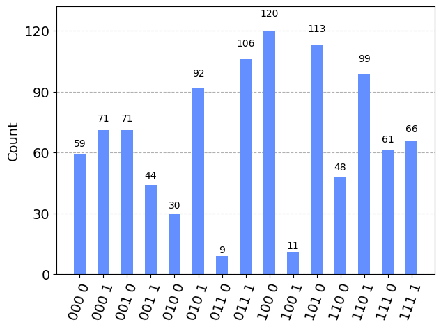
qsound_sqpam.run(shots)
print(qsound_sqpam.counts)
plot_histogram(qsound_sqpam.counts)
{'001 0': 71, '110 1': 99, '101 0': 113, '111 1': 66, '000 1': 71, '111 0': 61, '001 1': 44, '011 1': 106, '011 0': 9, '100 0': 120, '110 0': 48, '010 1': 92, '100 1': 11, '000 0': 59, '010 0': 30}
[17]:
QSM:
[18]:
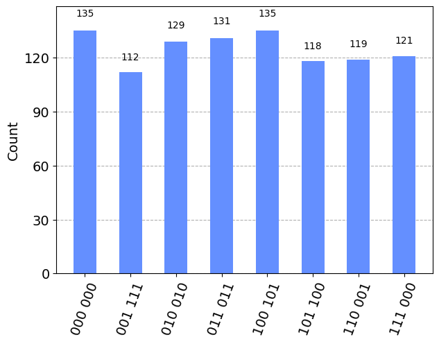
qsound_qsm.run(shots)
print(qsound_qsm.counts)
plot_histogram(qsound_qsm.counts)
{'010 010': 129, '110 001': 119, '111 000': 121, '100 101': 135, '001 111': 112, '011 011': 131, '000 000': 135, '101 100': 118}
[18]:
The last step of the process is to decode/reconstruct the histogram output into a digital audio output using the reconstruct_audio() method:
QPAM
[19]:
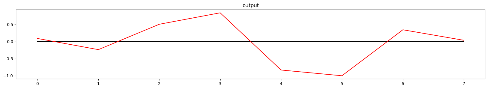
qsound_qpam.reconstruct_audio()
qsound_qpam.plot_audio()

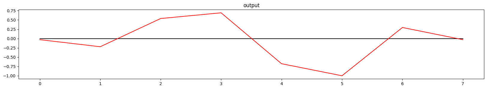
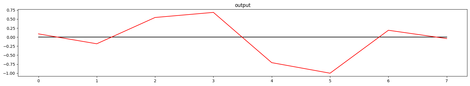
You might notice that the reconstructed signal is not perfect. This is the case for QPAM and SQPAM, as they have proabilistic retrieval characteristics. This means: The higher the amount of experiments (shots), the higher the precision of the reconstructed signal will be:
[20]:
qsound_qpam.output
[20]:
array([-0.03020621, -0.22025645,  0.53801821,  0.69100562, -0.6767354 ,
       -1.        ,  0.29672665, -0.03020621])
[21]:
qsound_qpam.input
[21]:
array([ 0. , -0.25, 0.5 , 0.75, -0.75, -1. , 0.25, 0. ])
[22]:
# Reconstrunction Error
sum(qsound_qpam.output - qsound_qpam.input)
[22]:
0.0683462015824361
SQPAM
[23]:
qsound_sqpam.reconstruct_audio()
qsound_sqpam.plot_audio()

QSM
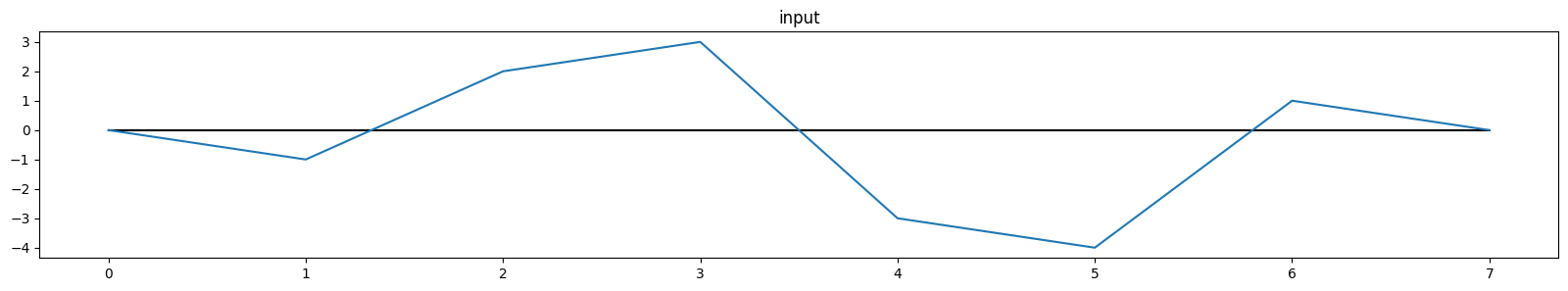
Note: QSM has a deterministic retrieval procedure, hence, perfect reconstruction
[24]:
qsound_qsm.reconstruct_audio()
qsound_qsm.plot_audio()
Finally, listen to the output with listen() (in this case, the output is too short to be heard):
[25]:
sample_rate = 3000
qsound_qpam.listen(sample_rate)
For one-liners, this whole process can be written, for any representation, as:
[26]:
qsound = qa.QuantumAudio('qpam')
qsound.load_input(quantized_ditial_audio, 3).prepare().measure().run(1000).reconstruct_audio().plot_audio()
For this input, the QPAM representation will require:
         3 qubits for encoding time information and
         0 qubits for encoding ampĺitude information.
This summarizes the introduction to the quantumaudio module. For more functionalities and potential applications, refer to the documentation and to the Github Repository Readme file.
.
.
Download this notebook from the latest Github release.
Itaborala @ ICCMR Quantum https://github.com/iccmr-quantum/quantumaudio